Cecilia's Site
My class work for bimm143 at UC San Diego
Lab 8: Mini-Project
Cecilia Wang (A18625854)
Background
In today’s class we will apply the methods and techniques clustering and PCA to help make sense of a real world breast cancer FNA biopsy data set.
Data import
We start importing our data. It is a CSV file so we will use read.csv
function.
fna.data <- read.csv("WisconsinCancer.csv")
wisc.df <- data.frame(fna.data, row.names=1)
head(wisc.df,2)
       diagnosis radius_mean texture_mean perimeter_mean area_mean
842302         M       17.99        10.38          122.8      1001
842517         M       20.57        17.77          132.9      1326
       smoothness_mean compactness_mean concavity_mean concave.points_mean
842302         0.11840          0.27760         0.3001             0.14710
842517         0.08474          0.07864         0.0869             0.07017
       symmetry_mean fractal_dimension_mean radius_se texture_se perimeter_se
842302        0.2419                0.07871    1.0950     0.9053        8.589
842517        0.1812                0.05667    0.5435     0.7339        3.398
       area_se smoothness_se compactness_se concavity_se concave.points_se
842302  153.40      0.006399        0.04904      0.05373           0.01587
842517   74.08      0.005225        0.01308      0.01860           0.01340
       symmetry_se fractal_dimension_se radius_worst texture_worst
842302     0.03003             0.006193        25.38         17.33
842517     0.01389             0.003532        24.99         23.41
       perimeter_worst area_worst smoothness_worst compactness_worst
842302           184.6       2019           0.1622            0.6656
842517           158.8       1956           0.1238            0.1866
       concavity_worst concave.points_worst symmetry_worst
842302          0.7119               0.2654         0.4601
842517          0.2416               0.1860         0.2750
       fractal_dimension_worst
842302                 0.11890
842517                 0.08902
# We can use -1 here to remove the first column
wisc.data <- wisc.df[,-1]
Remove the “diagnosis” line
diagnosis <-wisc.df[,1]
Exploratory data analysis
Q1. How many observations are in this dataset?
nrow(wisc.data)
[1] 569
Q2. How many of the observations have a malignant diagnosis?
length(grep("M",diagnosis))
[1] 212
# sum(wisc.df$diagnosis==M)
# table(wisc.df$diagnosis)
Q3. How many variables/features in the data are suffixed with _mean?
sum(grepl("_mean$", names(wisc.data)))
[1] 10
#length(grep("_mean"),colnames(wisc.data))
Principal Component Analysis
# Check column means and standard deviations
colMeans(wisc.data)
            radius_mean            texture_mean          perimeter_mean
           1.412729e+01            1.928965e+01            9.196903e+01
              area_mean         smoothness_mean        compactness_mean
           6.548891e+02            9.636028e-02            1.043410e-01
         concavity_mean     concave.points_mean           symmetry_mean
           8.879932e-02            4.891915e-02            1.811619e-01
 fractal_dimension_mean               radius_se              texture_se
           6.279761e-02            4.051721e-01            1.216853e+00
           perimeter_se                 area_se           smoothness_se
           2.866059e+00            4.033708e+01            7.040979e-03
         compactness_se            concavity_se       concave.points_se
           2.547814e-02            3.189372e-02            1.179614e-02
            symmetry_se    fractal_dimension_se            radius_worst
           2.054230e-02            3.794904e-03            1.626919e+01
          texture_worst         perimeter_worst              area_worst
           2.567722e+01            1.072612e+02            8.805831e+02
       smoothness_worst       compactness_worst         concavity_worst
           1.323686e-01            2.542650e-01            2.721885e-01
   concave.points_worst          symmetry_worst fractal_dimension_worst
           1.146062e-01            2.900756e-01            8.394582e-02
apply(wisc.data,2,sd)
            radius_mean            texture_mean          perimeter_mean
           3.524049e+00            4.301036e+00            2.429898e+01
              area_mean         smoothness_mean        compactness_mean
           3.519141e+02            1.406413e-02            5.281276e-02
         concavity_mean     concave.points_mean           symmetry_mean
           7.971981e-02            3.880284e-02            2.741428e-02
 fractal_dimension_mean               radius_se              texture_se
           7.060363e-03            2.773127e-01            5.516484e-01
           perimeter_se                 area_se           smoothness_se
           2.021855e+00            4.549101e+01            3.002518e-03
         compactness_se            concavity_se       concave.points_se
           1.790818e-02            3.018606e-02            6.170285e-03
            symmetry_se    fractal_dimension_se            radius_worst
           8.266372e-03            2.646071e-03            4.833242e+00
          texture_worst         perimeter_worst              area_worst
           6.146258e+00            3.360254e+01            5.693570e+02
       smoothness_worst       compactness_worst         concavity_worst
           2.283243e-02            1.573365e-01            2.086243e-01
   concave.points_worst          symmetry_worst fractal_dimension_worst
           6.573234e-02            6.186747e-02            1.806127e-02
# Perform PCA on wisc.data by completing the following code
wisc.pr <- prcomp(wisc.data,scale= T)
summary(wisc.pr)
Importance of components:
                          PC1    PC2     PC3     PC4     PC5     PC6     PC7
Standard deviation     3.6444 2.3857 1.67867 1.40735 1.28403 1.09880 0.82172
Proportion of Variance 0.4427 0.1897 0.09393 0.06602 0.05496 0.04025 0.02251
Cumulative Proportion  0.4427 0.6324 0.72636 0.79239 0.84734 0.88759 0.91010
                           PC8    PC9    PC10   PC11    PC12    PC13    PC14
Standard deviation     0.69037 0.6457 0.59219 0.5421 0.51104 0.49128 0.39624
Proportion of Variance 0.01589 0.0139 0.01169 0.0098 0.00871 0.00805 0.00523
Cumulative Proportion  0.92598 0.9399 0.95157 0.9614 0.97007 0.97812 0.98335
                          PC15    PC16    PC17    PC18    PC19    PC20   PC21
Standard deviation     0.30681 0.28260 0.24372 0.22939 0.22244 0.17652 0.1731
Proportion of Variance 0.00314 0.00266 0.00198 0.00175 0.00165 0.00104 0.0010
Cumulative Proportion  0.98649 0.98915 0.99113 0.99288 0.99453 0.99557 0.9966
                          PC22    PC23   PC24    PC25    PC26    PC27    PC28
Standard deviation     0.16565 0.15602 0.1344 0.12442 0.09043 0.08307 0.03987
Proportion of Variance 0.00091 0.00081 0.0006 0.00052 0.00027 0.00023 0.00005
Cumulative Proportion  0.99749 0.99830 0.9989 0.99942 0.99969 0.99992 0.99997
                          PC29    PC30
Standard deviation     0.02736 0.01153
Proportion of Variance 0.00002 0.00000
Cumulative Proportion  1.00000 1.00000
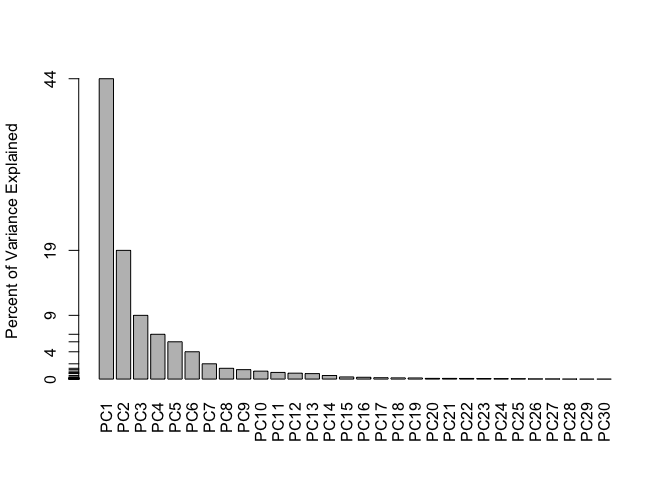
Q4. From your results, what proportion of the original variance is captured by the first principal component (PC1)?
44.27%
Q5. How many principal components (PCs) are required to describe at least 70% of the original variance in the data?
PC3 a captured 72.6% variance
Q6. How many principal components (PCs) are required to describe at least 90% of the original variance in the data?
PC7 already captured 91% variance
Interpreting PCA results
biplot(wisc.pr)
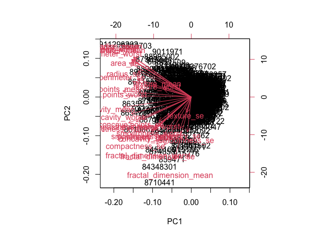
This plot is very hard to read and understand
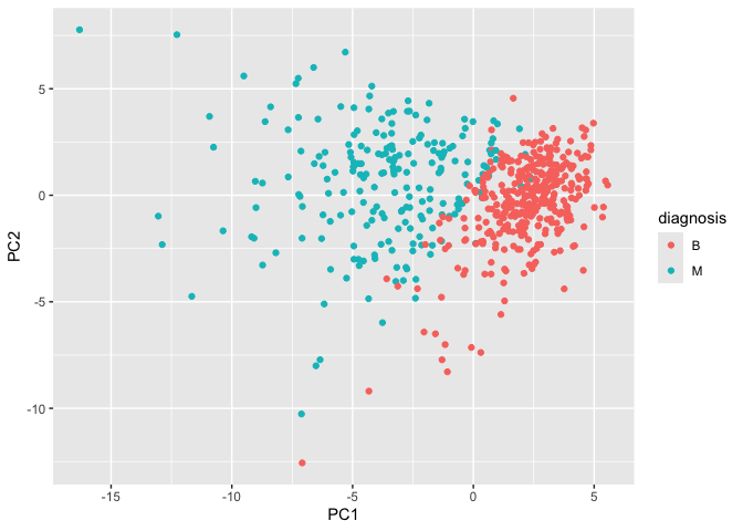
Scatter plot: PC1 vs. PC2
# Scatter plot observations by components 1 and 2
library(ggplot2)

ggplot(wisc.pr$x) +
  aes(PC1, PC2, col=diagnosis) +
  geom_point()
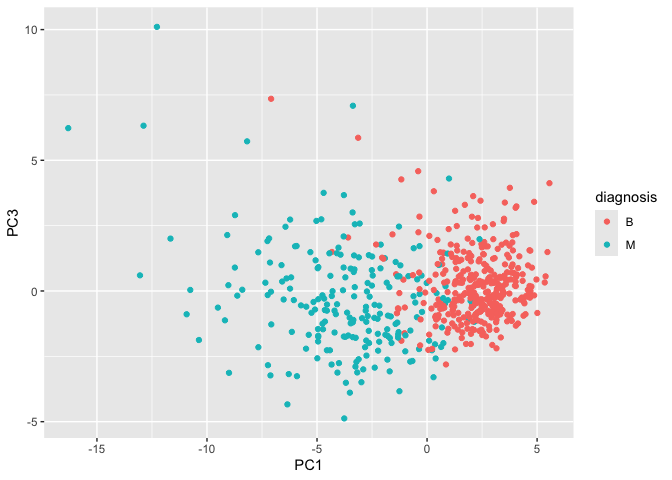
Scatter plot: PC1 vs. PC3
library(ggplot2)

ggplot(wisc.pr$x) +
  aes(PC1, PC3, col=diagnosis) +
  geom_point()
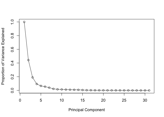
Variance explained
# Calculate variance of each component
pr.var <- wisc.pr$sdev^2
head(pr.var)
[1] 13.281608 5.691355 2.817949 1.980640 1.648731 1.207357
# Variance explained by each principal component: pve
pve <-pr.var/30

# Plot variance explained for each principal component
plot(c(1,pve), xlab = "Principal Component",
     ylab = "Proportion of Variance Explained",
     ylim = c(0, 1), type = "o")
# Alternative scree plot of the same data, note data driven y-axis
barplot(pve, ylab = "Percent of Variance Explained",
     names.arg=paste0("PC",1:length(pve)), las=2, axes = FALSE)
axis(2, at=pve, labels=round(pve,2)*100 )
Communicating PCA results
Q9. For the first principal component, what is the component of the loading vector (i.e. wisc.pr$rotation[,1]) for the feature concave.points_mean? This tells us how much this original feature contributes to the first PC. Are there any features with larger contributions than this one?
wisc.pr$rotation["concave.points_mean",1]
[1] -0.2608538
Hierarchical clustering
# Scale the wisc.data data using the "scale()" function
data.scaled <- scale(wisc.data)
data.dist <- dist(data.scaled)
wisc.hclust <- hclust(data.dist)
plot(wisc.hclust)
abline(h=19.5, col="red", lty=2)
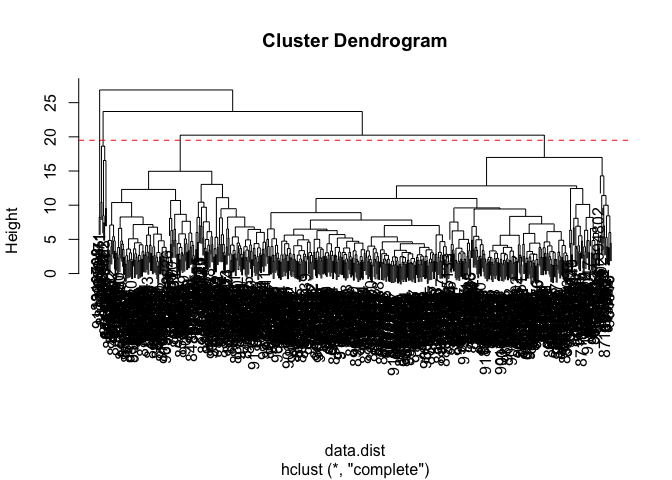
wisc.hclust.clusters <- cutree(wisc.hclust,k=4)
table(wisc.hclust.clusters, diagnosis)
                    diagnosis
wisc.hclust.clusters   B   M
                   1  12 165
                   2   2   5
                   3 343  40
                   4   0   2
Combine methods
Here we will take our PCA results and use those as input for clustering.
In other words our wisc.pr$x scores that we plotted above (the main
output from PCA - how the data lie on our new principal component
axis/variables) and use a subset of these PCs that captre the most
variance as input for hclust().
wisc.pr.hclust <-hclust(dist(wisc.pr$x[,1:3]), method = "ward.D2")
plot(wisc.pr.hclust)
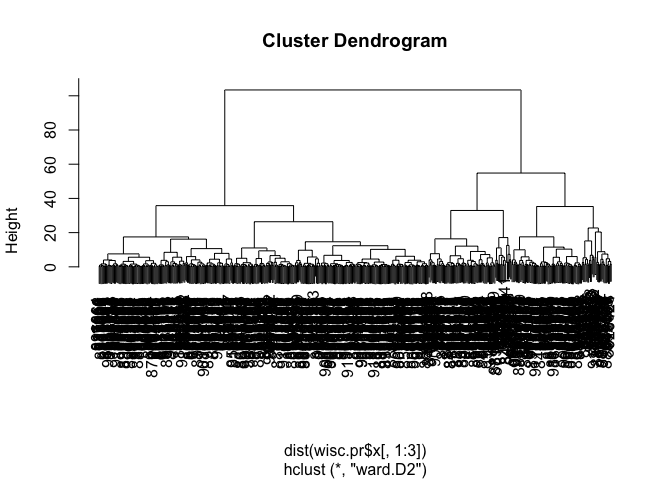
Cut the dendrogram/tree into two main groups/clusters:
grps <- cutree(wisc.pr.hclust, k=2)
table(grps)
grps
  1   2
203 366
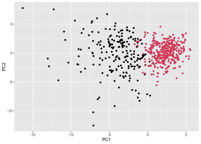
I want to know how the clustering in grps with values of 1 or 2
correspond the expert diagnosis
table(grps, diagnosis)
    diagnosis
grps   B   M
   1  24 179
   2 333  33
My clustering group 1 are mostly “M” diagnosis (179) and my clustering group 2 are mostly “B” diagnosis (333)
24 FP 179 TP 333 TN 33 FN
Specificity: TP/(TP+FN)
179/(179+33)
[1] 0.8443396
Specificity: TN/(TN+FP)
333/(333+24)
[1] 0.9327731
ggplot(wisc.pr$x) +
  aes(PC1, PC2) +
  geom_point(col=grps)
Prediction
#url <- "new_samples.csv"
url <- "https://tinyurl.com/new-samples-CSV"
new <- read.csv(url)
npc <- predict(wisc.pr, newdata=new)
npc
           PC1       PC2        PC3        PC4       PC5        PC6        PC7
[1,]  2.576616 -3.135913  1.3990492 -0.7631950  2.781648 -0.8150185 -0.3959098
[2,] -4.754928 -3.009033 -0.1660946 -0.6052952 -1.140698 -1.2189945  0.8193031
            PC8       PC9       PC10      PC11      PC12      PC13     PC14
[1,] -0.2307350 0.1029569 -0.9272861 0.3411457  0.375921 0.1610764 1.187882
[2,] -0.3307423 0.5281896 -0.4855301 0.7173233 -1.185917 0.5893856 0.303029
          PC15       PC16        PC17        PC18        PC19       PC20
[1,] 0.3216974 -0.1743616 -0.07875393 -0.11207028 -0.08802955 -0.2495216
[2,] 0.1299153  0.1448061 -0.40509706  0.06565549  0.25591230 -0.4289500
           PC21       PC22       PC23       PC24        PC25         PC26
[1,]  0.1228233 0.09358453 0.08347651  0.1223396  0.02124121  0.078884581
[2,] -0.1224776 0.01732146 0.06316631 -0.2338618 -0.20755948 -0.009833238
             PC27        PC28         PC29         PC30
[1,]  0.220199544 -0.02946023 -0.015620933  0.005269029
[2,] -0.001134152  0.09638361  0.002795349 -0.019015820
plot(wisc.pr$x[,1:2], col=grps)
points(npc[,1], npc[,2], col="blue", pch=16, cex=3)
text(npc[,1], npc[,2], c(1,2), col="white")
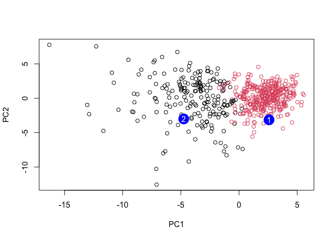
Q. Which of these new patients should we prioritize for follow up based on your results?
Patient 1 should be prioritize.